


treatability tests
Reading time:study of natural sedimentation and desludging
Waters that have a high suspended solids content (over 2 g · L-1) often require a preliminary coarse screening.
Sedimentation in test tubes is monitored versus time to evaluate particle sedi- mentation rates. Suspended solids concentrations in the clarified water and in the settled sludge are measured to determine the volume of sludge produced and its concentration. Should a reagent be added its action should be simulated in a laboratory flocculator (see below).
study of water coagulation and flocculation
The objective is to investigate the type and amounts of reagents required to treat water under optimum conditions (see coagulation-floculation)
- adding coagulants and flocculants;
- adjusting pH;
- dosing powdered adsorbent ( PAC ).
The addition of oxidants is recommended (chlorine, ozone, chlorine dioxide). The amount of coagulant required can be established either by electrophoresis or by flocculation tests also known as “jar-tests”.
electrophoresis
This technique consists in observing the movement of colloids placed in an electrical field. The apparatus used to carry out this measurement (the Zetameter) comprises a control unit, an electrophoresis cell, a lighting arrangement, a binocular microscope suitable for viewing the particles that measure approximately one micron. Colloid movement can be measured manually or automatically. Determination is first carried out on raw water and then with increasing amounts of coagulant. The Zeta potential of colloid particles can be calculated from their rate of movement and temperature (please refer to apparatus operating instructions).
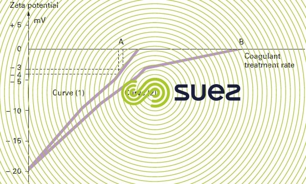
The change in potential (expressed in millivolts) versus the amount of coagulant used can be plotted (see figure 7 below). For waters that match curve 1 (primarily colloidal turbidity), amount A of the reagent is required to achieve a – 3 to – 4 millivolt potential. On the other hand, for waters with a high content of algae or OM that match curve 2, amount B is required to cancel out the Zeta potential.

Transporting water samples from the site to the laboratory has little impact on the result of an electrophoresis analysis.
flocculation test: jar-test
In addition to determining the amount of coagulant required, these tests can be used to visualize the flocculation process and ascertain its effects on both clarified water and sludge. These tests must be carried out at a temperature close to that of the actual water undergoing treatment in the field.
First, varying amounts of the flocculation reagent are tested. If the result obtained is insufficient a new series of tests is conducted repeating the conditions that previously provided the best results and experimenting with different doses. When using several reagents, the injection sequence and the time sepa- rating each injection should be taken into account.
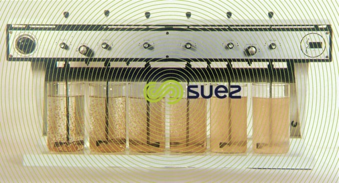
It is recommended to use a flocculator that can stir a series of beakers simultaneously and at a very precise rotation speed to achieve comparable results. It is crucial that the revolutions per minute and subsequently the speed gradien be identical inside all the beakers. The optimum rotation speed is in the region of 40 revolutions per minute for a 1 x 5 cm blade rotating inside a 1-liter beaker.
This test is carried out for 20 minutes and the following information should be recorded:
- amounts of reagents used and injection sequence;
- flocculation appearance expressed as follows:
- 0: no floc;
- 2: floc barely visible, small dots;
- 4: small floc;
- 6: medium size floc;
- 8: good floc;
- 10: very large floc (> 1 cm);
- pH after flocculation.
For the best obtained results, this data is supplemented with the following information:
- color and turbidity of the clarified water;
- percentage sludge sedimentation;
- flocculent settling rate;
- sludge cohesion coefficient or sludge sedimentation rate;
- clarified water permanganate oxidation capability;
- measurements specific to the treatment under examination: Fe, Mn, TOC, micro algae, specific pollutants …
sedimentation analysis
An electrophoresis study followed by a flocculation test are insufficient to safely extrapolate results to a full-scale system. Since the main purpose is to know at what rise rate a clarifier should be operated a sedimentation study is also required.
There are two possible cases:
- sparse flocculation: if the flocculated water is allowed to rest, each particle deposits as if it was alone existed in isolation, some at a faster rate, others slower. The liquid clarifies gradually and a deposit forms at the bottom of the beaker. This is known as free or diffused sedimentation;
- intense flocculation: sedimentation involves all the flocculated particles, cre- ating a layer of clear liquid above a sludge layer inside the beaker. This is termed hindered settling and it occurs when treating waters that contain an abundant amount of setteable solids.
The measurements required are different whether sparse or intense flocculation occurs.
measuring sludge cohesion
For diffused sedimentation, adding increasing amounts of sludge results in the settling velocity to increase. This occurs until the liquid contains a sufficient amount of sludge to induce hindered settling. This observation is the basis of the industrial use of “sludge contact” or sludge blanket clarification.
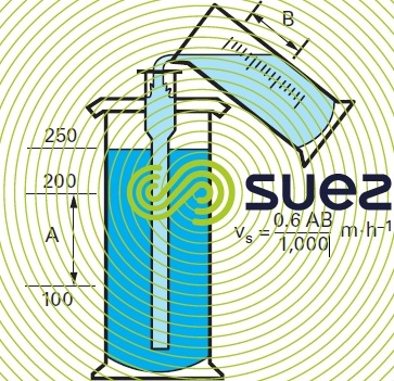
When a layer of sludge is subjected to a rising current of water it expands and occupies an apparent volume that is proportional to the rising rate of velocity. This phenomenon characterises the sludge cohesion. In a 250 mL test tube, identical to the one shown in figure 9, place sludge collected from several beakers used during a flocculation test, each beaker having been injected with the same amount of reagents. Allow the sludge to rest for 10 minutes. Siphon off the excess sludge until all that is left in the test tube is an apparent volume of approximately 50 mL.
Then insert into the test tube a long-stem funnel such that the end of the stem is located approximately 10 mm above the bottom of the test tube. Slightly sink the funnel through the water menisque at the top of the test tube to prevent the introduction of air bubbles. Add water into the funnel using settled water obtained during flocculation tests to avoid any pH or temperature gradient problems. The water should be added progressively in small amounts, as any excess would result in the test tube to overflow.
Adding water in the manner described above results in the sludge bed to expand. The water rising velocity can be calculated for various sludge expansion rates.
Measure the time T (in seconds) that is required for 100 mL of water to expand the sludge bed to apparent volumes of 100, 125, 150, 175, 200 mL.
To calculate the velocity v, if A is the height of the test tube in millimetres for 100 mL (distance separating the 100 and 200 mL markings on a 250 mL test tube), v is equal to 3.6 A/t m.h-1
The results can be plotted on a graph by entering v along the Y-axis and V along the X-axis (figure 8).
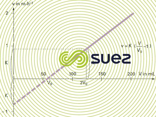
It is clear that the curve representing velocity variations as a function of the expanding volume of sludge is in fact a straight line.


v: rising velocity in the test tube needed to obtain the volume V,
V: apparent volume of the expanding sludge,
V0: volume of the compacted sludge at zero velocity and measured on the graph.
The coefficient “K” is the characteristic of the cohesion of the sludge, it is called the sludge cohesion factor. Since the K factor is temperature-dependent the water temperature should be carefully recorded during testing.
For a sludge that is cohesive and quick to settle the K factor can reach values of 0.8 to 1.2.
Conversely, a watery sludge that contains fragile and light flocs yields much lower K values, typically not exceeding 0.3. Therefore, measuring the K factor provides extremely valuable information on how the precipitate would behave in a “sludge contact” clarifier. It also helps establishing the impact of flocculant addition.
There is often no link between the size of the flocs and sludge cohesion
measuring hindered settling rate
When the flocculation test results in “hindered settling” enriching the liquid with sludge is pointless and may even be harmful.
The aim is to directly measure the contraction rate of the sludge as produced during the flocculation tests and as it would naturally occur in an industrial scale clarifier.
Process is the same that for the sludge cohesion coefficient K measurement but at a concentration equal to that obtained from flocculating 1 liter of test water.
A 250 mL test tube is filled with the flocculated liquid. The sludge is allowed to settle for 5 to 10 minutes to allow the floc to reform. Using a long-stem funnel introduce water resulting in the sludge bed to expand until it reaches an apparent volume of 250 mL.
The rate recorded indicates the rising velocity that would be possible in an industrial clarifier. It is the rate shown by the linear section of the Kynch curve (see different types of sedimentation).
Once this operation has been completed, it is suggested to let the sludge rest and compact in the test tube, recording the apparent volumes versus time (from 0 to 2 hours). This measurement gives an indication of the volume of sludge that needs to be extracted in an industrial size clarifier. Accordingly, the clarifier sludge handling parts can then be sized (sludge collection pits, scraper blades).
Figure 9 summarises the operations involved:
- test tube height for 100 mL (A mm);
- volume of water introduced in 1 minute in order to maintain the upper level of the sludge at the same level of the liquid introduced into the test tube (250 mL) (B mL);
- theoretical settling rate in metres vs m · h‑1.
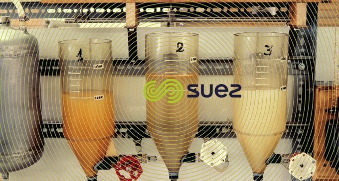
flotation test – flottatest (photo 5)
Using a pressurised water tank, introduce increasingly large volumes of pressurised water into the various beakers where optimum flocculation of the untreted water first took place. The following data should be logged:
- % pressurised water;
- bubble rising velocity;
- floc rising velocity;
- floc appearance;
- sludge cake thickness;
- measurements carried out on floated water: turbidity, colour, OM …;
- sludge resistance and suitability for scraping
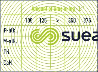
carbonate removal test using lime
Typically, the coagulant used is ferric chloride but aluminum sulphate can also be tested with or without additives. In this case, the aluminum concentration is measured following filtration through paper (aluminium is very soluble in an alkaline medium).
A first test is carried out without coagulant to establish the amount of lime required while injecting 10 g per litre of powdered CaCO3 (granulometry 50 µm). Stir for 5 minutes prior to settling and filtering through a slow filtration paper filter. Titer the filtered water and compute the results in a table (table 4).
Then, using the amount of lime that resulted in either an alkalinity above 0.5 °F at half the total alkalinity or a minimum hardness, repeat the flocculation test but using increasing amounts of coagulant.
For silicon removal, another reagent (magnesium oxide, aluminate…) can be used and silicon content measured on filtered water. For water softening applications sodium carbonate should be used.
determination of oxidizing agent demands
chlorine absorption test (chlorine demand)
Use a set of flasks all having the same voume capacity and made of glass with identical composition.
Introduce the same amount of test water into each flask and add increasing amounts of chlorine. Following a contact time that is identical to the water residence time in the installation, measure the free chlorine concentration in each flask. Note that measurement should be performed at a steady temperature and away from light (for some studies it is recommended to carry out this research with different contact times: 1, 2, 5… 24 hours).
A curve of residual chlorine concentration versus the amount of chlorine injected (see oxidation and reduction, figure 93).
It is strongly recommended that both total and free chlorine concentrations be analysed, especially when the chlorine absorption curve does not display a critical point. As a result, the chlorine demand for a given set of contact times can be established. Additional specific measurements can be undertaken based on increasing amounts of chlorine: formation of haloforms, color, organic matter, effect on flocculation, taste thresholds.
quick method for determining the critical point
This method consists of taking one single measurement, by injecting into the raw water a largely excessive amount of chlorine (E in figure 93 of oxidation and reduction); after contact, a measurement of the residual chlorine, can be used to produce an approximation of the breakpoint value, viz. E – e.
operating test chlorine absorption kinetics curve for treated water
For a given amount of chlorine injected, free and total chlorine concentrations are logged versus time. The sections of the curve that require an in-depth examination apply to the “rapid demand” (less than one hour) and to consumption after a lengthy contact time (long networks). This test can provide information on the validity of re-chlorination carried out at different points on a water distribution network.
chlorine dioxide absorption test
Ascertaining the chlorine dioxide demand of a water requires the same procedure as that used to assess the chlorine demand: the disinfectant residual is plotted versus the amount injected. In the presence of ammonia, the curve has no critical point (because chlorine dioxide does not react with the ammonium cation). A concentrated solution of chlorine dioxide is prepared from sodium chlorite in the presence of an excess of hydrochloric acid.
The stock solution should have a concentration of approximately 15 g· L-1 CℓO2. The dilute solution is usually prepared for 0.5 g· L-1. This concentration should be checked along with the absence or presence of chlorite.
ozone absorption test
In the laboratory or in the field, a water’s ozone demand is determined using a special flask (figure 10).
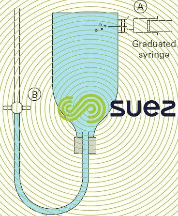
Ozonated air is injected at A using a graduated syringe. When tap B is opened, a volume of air identical to the volume of ozone is displaced.
When tap B is closed, the flask is shaken by hand for the same period of time as the water contact time in the ozone contactor. The residual ozone is then measured by titrimetry using diethylphenylene diamine ( DPD ) following addition of potassium iodide.
The following formula calculates the amount of ozone injected:

where :
C03 : ozone concentration in the carrier gas expressed in mg · L-1,
V: flask capacity (L), v: volume of ozonated gas (L)
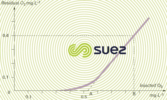
The residual ozone concentration is then plotted versus the amount of ozone injected. A curve with the following typical points should be obtained (see figure 11 below):
- point A where the extended line intersects the X-axis, representing the amount of ozone that needs to be injected in order to meet the water’s chemical demand for ozone and to generate residual ozone;
- point B is the line that represents the amount of ozone that has to be injected in order to meet the ozone demand and to obtain the target residue, after the contact time selected, e.g. 0.4 mg · L-1.
degassing-aeration test
It is sometimes necessary to flush residual CO2 out of a water by trickling it through air. With the goal to check the effectiveness of this operation take two 1 L beakers and pour water from one beaker into the other respecting a 20 cm height, at a rate of approximately 1 liter in 10 sec. Residual CO2 concentration and pH should be measured and recorded versus the number of pours until the pH stabilises.
physical-chemical iron removal test
Iron removal by air oxidation is not always feasible, especially with OM rich waters. In order to check this a test is required. This test should be carried out on the spot, immediately following samples collection:
- rapidly aerate the sample by transferring it twenty times from one beaker into another;
- filter the sample through Durieux paper, a blue strip filter or an 0.45 µm membrane;
- check the amount of residual iron, the change in pH , in dissolved oxygen and in carbon dioxide.
If the residual amount of iron is greater than 0.1 mg · L-1, additional testing is required, if possibly using a pilot unit or other oxidants and/or various coagulants and flocculants (e.g. alginates).
Bookmark tool
Click on the bookmark tool, highlight the last read paragraph to continue your reading later
