


methods used to determine pHS
Reading time:ions present
We have:
- "constituent ions": H+, or better still H3O+ because it is a hydrated ion, and OH–;
- the other fundamental ions: Ca2+, HCO3–, CO32–;
- secondary ions: Na+, K+, Mg2+, Fe2+… Cℓ–, SO42–, NO3–, SiO32–…
the equilibriums and their thermodynamic constants
Among these ions, four major equilibriums govern the reciprocal concentrations:
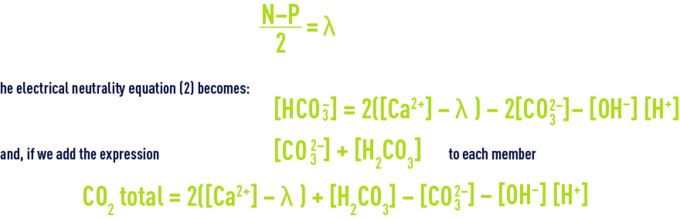
- a) equal positive and negative electrical charges (electrical neutrality equation):


that can also be written:

P and N represent respectively Mg, K and Na concentrations on the one hand and Cℓ, NO3 et SO4 concentrations on the other.
Note: Fe, Mn, SiO2… are elements termed "minor" and their concentration can be regarded as negligible compared to that of the other elements.
- b) water ionisation:

- c) carbonic acid dissolution and dissociation:
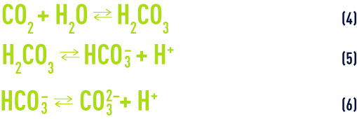
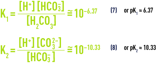
At temperature of 25°C and in the absence of any other dissolved salts, the law of mass action applied to equilibriums (5) and (6) (see section ionisation) gives us:
- d) calcium carbonate dissolution/precipitation balance:

Notes:
Other states of equilibrium may occur and bring weak acids into play: this applies to SiO2 and to H2S or to humic acids; we shall not take these into consideration as they represent special cases.
The above thermodynamic constants are subject to major variations depending on temperature (table 45).
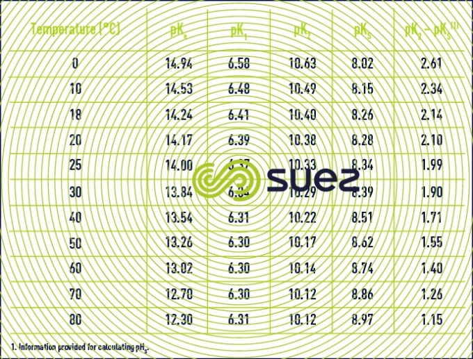

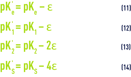
- For practical reasons, the figures provided in table 45 apply to apparent constants (Debye & Hückel), based on the concentrations (deduced from analyses and expressed as mol/L) of the various ions and not on their activity; additionally, they also depend on water salinity; this effect can be evaluated in the form of a magnitude termed the ionic force, designated by µ, expressed in moles per litre and defined by the following equation :to apply an ionic force correction to the different pK’s :
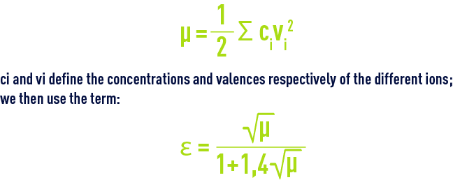
- A few outline figures for Ɛ (if we do not have a complete ionic balance, Ɛ can also be deduced from the resistivity) are provided in table 46 :
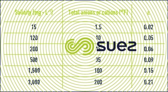
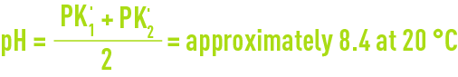
Table 46. A few examples of the magnitude of the term ε - These equations show us that a water’s pH is directly dependant on its relative levels of free CO2 on the one hand and on the HCO3– and CO32- ions (i.e. alkalinity measured by the M-alk. ) on the other; in particular, the following can be deduced from equations (7) and (12) :
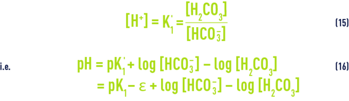
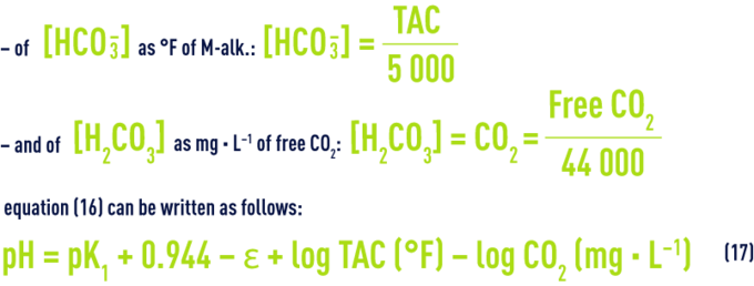
Earlier, we discussed values for pK1 based on temperature and on e as a function of salinity; furthermore, in water having a pH below 8.4 (the case for most natural waters), we can ignore the CO32– ion levels and assume that the M-alk. relates exclusively to the HCO3– ions; finally, [H2CO3] refers to the total free CO2 measured because we cannot measure non-dissociated carbonic acid H2CO3 and carbon dioxide CO2 dissolved in water, separately.
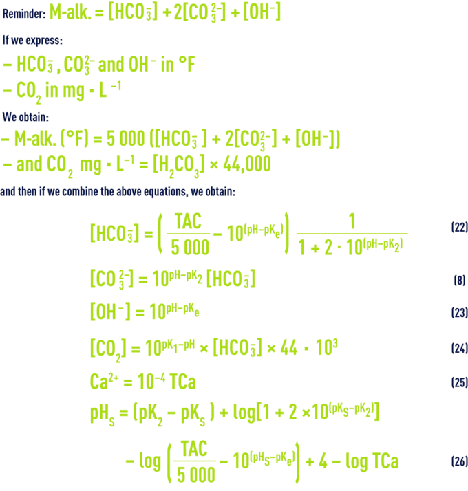
Consequently, whatever the water, there is a close link between pH, M-alk. and free CO2; after we have transposed the concentrations into mo l· L–1:
pHS approximation through calculation
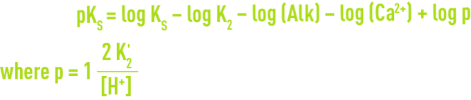
When water is at the state of calcium-carbonate balance (neither aggressive nor scale-forming, see section treatment objectives), this means that it is CaCO3 saturated and that CO32– andCa2+ ion concentrations (expressed in mo l· L–1) satisfy the solubility product (10) that can also be written:

If we write this equation in yet another way, we will know that a water is in the state of calcium-carbonate balance when:
Values for pK2 – pKS (based on temperature) and of e (based on salinity) can be taken direct from the above tables 45 and 46. As e, pHS rises with salinity and, therefore, this becomes an important factor for brackish water (salinity > 1 g · L–1).
Using the M-alk. and the CaH (°F), for water having a pH < 8.4 approximately, this equation then becomes:

We have already seen that when pH < pHS, water tends to dissolve limestone (aggressivity); when pH is too low, this is caused by an excess of dissolved carbon dioxide; the fraction of carbon dioxide that is likely to react with calcium carbonate is termed aggressive CO2. The CO2 concentration that is precisely right at pHS is termed the balancing CO2(in the sense of chemical saturation (1) discussed under ; the total dissolved free CO2 content will, therefore, be equal to the sum of: balancing CO2 + excess CO2(of which part is CO2 that attacks limestone, shifting the balance to the left).
On the other hand, water having a pH > pHS is scale-forming: it is lacking in dissolved CO2 and tends to compensate by shifting balance (1) to the right with precipitation of CaCO3.
approximation of pHS using graphs
general
Numerous authors have expanded on their respective methods: Franquin & Marécaux, Tillmans, Hallopeau & Dubin, Legrand & Poirier are some of the best known authors.
The aim remains the same: establishing a plan showing the axes linked to a parameter (pH) or to a sum of parameters (M-alk., total CO2) and, using this plan, plotting the representative location where water is in the state of calcium-carbonate balance: this location, termed "equilibrium curve", divides the plan into two sections, the aggressive (pH < pHS) water and the scale-forming water (pH > pHS).
As a reminder, it is to Tillmans that we owe the concept of protecting metals by using a protective film of iron and calcium carbonates (whence the name of Tillmans film).
the Langelier diagram
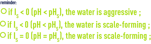
Langelier introduced the notion of pH compared against pHs resulting in the Langelier index: ILor IS (Saturation index) = pH – pHS; therefore: IS = 0: water in the state of equilibrium, IS < 0: aggressive water, IS > 0: scale-forming water.
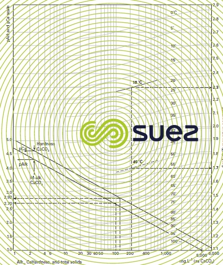
In order to determine this pHS, Langelier drew up a graph showing alkalinity and calcium expressed in mg · L–1 of CaCO3, and total salinity (dry extract in mg · L–1).
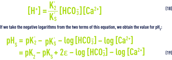
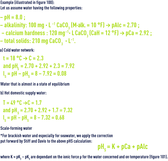
The following equation is used to deduce pHs from the diagram (figure 100):

This diagram allows for temperature and for salinity up to approximately 3 g·L–1 m but is not suitable for the calculation of amounts of "neutralisation" reagents.

Hallopeau and Dubin method
These authors have devised a graphic method that allows them to quantitatively characterise a water’s free CO2 content and its fraction that attacks limestone, to calculate the amounts of neutralisation reagents and to anticipate water properties after applying a correction to adjust the pH to the calcium-carbonate balance value.
By expressing the equilibrium pH as a function of alkalinity logarithms (alkalinity measured by the M-alk. and expressed as mol · L–1) and of calcium hardness (in mol · L–1), we obtain:
In this graph (figure 102), free CO2 and equilibrium pH will then be represented by two groups of parallel lines. For a given water, pHS will be determined by the intersection of:
- the vertical line drawn from representative point M, defined by the water’s M-alk. and pH;
- and the line parallel to the line for "CaCO3 saturation at 15 °C ", drawn from the water’s representative point in the left hand auxiliary diagram, containing values from the M-alk./CaH.
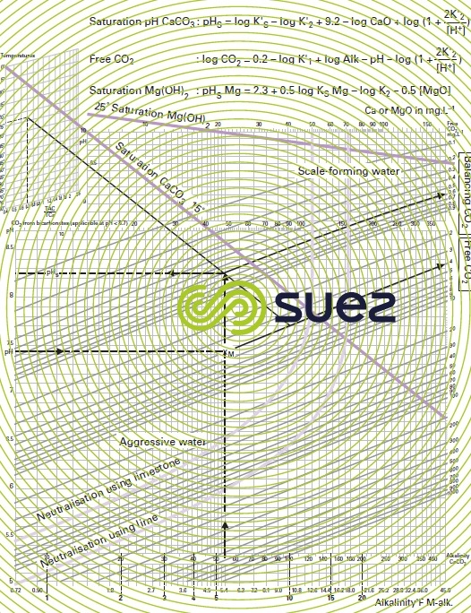
If point M is already on that line, water will be in a state of calcium-carbonate balance; below that line, it will be aggressive and, above it, scale-forming.
The graph also provides the pHS applicable to Mg(OH)2 precipitation at 25°C, i.e:

If we know a water’s pH and alkalinity, we can also determine its free CO2 and saturation CO2 (on the right hand scale, following it parallel to the system of oblique straight lines). The graph highlights the CO2 dissolution or physical loss curves and the lime (or sodium hydroxide) or calcium (or Na2CO3) neutralisation curves: the latter are obtained by plotting, starting from the water’s representative point, a curve that is parallel to the relevant base curve, as obtained through parallel translation in relation to the x-axis.
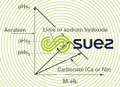
Figure 103 provides the example of a water whose representative point M, defined by its coordinates (M-alk., pH) is located in the aggressive zone: there are 3 possible ways of bringing this water into the state of equilibrium:
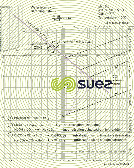
- n° 1: CO2 loss through aeration; M-alk. and calcium remain unchanged, the equilibrium pH is then the same as the pHS in the original water (in fact, this is rarely achievable excluding the case of a high M-alk. where the saturation CO2 is sufficiently high):
- n° 2: neutralisation using a base; M-alk. will rise and, when lime is used, calcium will also rise in the same proportion;
- n° 3: neutralisation using a carbonate (CaCO3 or Na2CO3); the M-alk. and, if applicable, the calcium (in the case of CaCO3) increase by about twice as much as in the previous example.
We can see that, on the one hand, equilibrium pH will be different in the 3 cases studied and that, on the other, the higher the final M-alk., the lower the pH equilibrium.
In cases n° 2 and 3, the difference between the final M-alk. and the initial M-alk. can be used to calculate the amount of alkaline reagent that needs to be used after evaluating the shift in the equilibrium line associated with the change affecting the alkalinity/calcium ratio as neutralisation takes place.
Although this method introduces total and calcium hardness concepts, it does not allow for total salinity and is only applicable to low to medium mineralisation water.
Legrand & Poirier method
These authors have examined a system with the coordinates along the X-axis and "total CO2" along the Y-axis (figure 104).
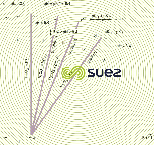
They support this choice on the ground of its advantages: the scales used are arithmetical (in principle in millimoles · L–1), which allows them to avoid origins that disappear from the scale; concentrations of all fundamental elements are immediately visible; the shift in the water’s figurative point almost always takes place along straight lines or along an equilibrium curve; finally, on this graph, treatment practicalities can be seen either as a shift of the figurative point or as a change to the equilibrium curve, or by both simultaneously.
Let N and P represent the respective sums of positive and negative secondary ions , and by postulating
By adopting the coordinates detailed above, we obtain a graph where the plan is divided into zones that are delineated by the main special cases (relating to the group of pH = constant curves which is one of the group of lines converging on point S of abscissa l); figure 104 identifies these zones: it is obvious that, in practice, almost all natural waters (before or after treatment) fall within zone III, i.e. between the line having a slope 4 (relating to pH = pK1' = approximately 6.4 at 20 °C) and to the line having a slope 2 that relates to:
The curve on which all calcium-carbonate balance waters can be found, for the temperature and parameter l values provided, will be of the type shown in figure 105; additionally, this figure provides examples of the figurative point M for a given water that is aggressive in view of its position in relation to the equilibrium curve and to the data that we can obtain from that curve with regard to the properties of the water (especially the proportion of aggressive CO2 as part of the total free CO2 content).

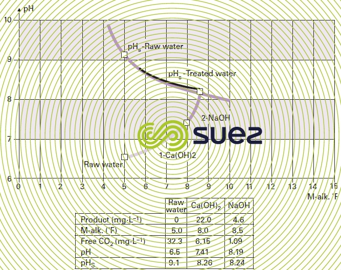
Degrémont® method : "Calcograph"
This method is derived from the Hallopeau & Dubin concept where water is shown on a pH = f (M-alk.) diagram but with linear scales.
The software then calculates:
- CO2 from the pH and the M-alk., or pH from the CO2 and from the M-alk. (equations 22 and 24);
- pHS from the M-alk. and from the CaH (equation 26).
The program allows for the variations of the various pK according to temperature and to the water’s ionic concentration (table 45 and equations 11 to 14).
We can then identify the figurative point for a water (through its pH and its M-alk.) and plot the curve for waters having a pH equal to pHS, for variable M-alk.'s: this is the "carbonate equilibrium curve" (or pHS-Raw water).
Each time a reagent is added, the software redefines the new parameters and represents the new figurative point, the path followed and the new pHS designated pHS-Treated water, whence the name Calcograph (figure 106).
correction options applicable to aggressive water - indices
We saw, earlier definitions of the various forms of CO2: free, excess, aggressive, saturation. As we know that there are 3 ways of reinstating the balance of an aggressive water (figure 103), figure 107 and table 47 provide the 3 final pHS and, therefore, 3 different balancing CO2 (calculated by the program and shown on the last line of the table).
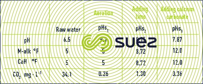
From the above, we can deduce the different expressions for excess CO2:
- aeration at constant M-alk.: 34.1 – 0.26 = 33.84 mg · L–1 of CO2 to be stripped;
- neutralisation using lime: 34.1 – 1.3 = 32.80 mg · L–1 of CO2 to be neutralised;
- neutralisation using CaCO3: 34.1 – 3.36 = 30.74 mg · L–1 of CO2 aggressive with regard to CaCO3; by definition, the «marble test» is the method used experimentally to access aggressiveCO2 with regard to limestone: in France it is expressed in "mg CO2 · L–1", and in Anglo-Saxon countries in "mg · L–1 of solubilisable CaCO3").

indexes
Attempts have often been made to characterise water in relation to the calcium-carbonate balance (with particular attention paid to aggressive water) and to its behaviour to ferrous metals by using a range of indexes of which the most frequently used are :
- the Langelier index orsaturation index:
IL = IS = pH – pHS ;
- the Larson index is the ratio between strong acid salts and hydrogen carbonate ions (see section treatment objectives) ;
- the Ryznar index defined by:
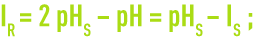
This index is always positive. Depending on its value, water trends can be determined by experimentation (at temperatures between 0 and 60°C) using the following scale :
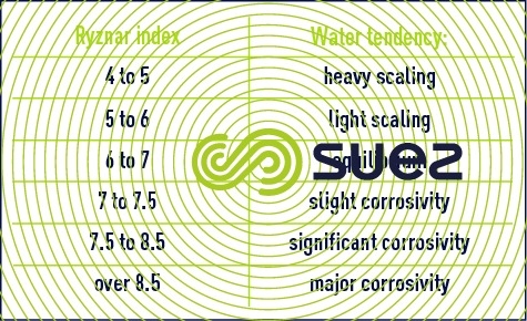
The purpose of aggressivity neutralisation consists primarily in cancelling out the Langelier index if it is negative at the outset; the Larson index shows that the higher the index, the more corrosive the water and this factor may call for particular measures (setting to IS > 0, remineralisation…); by examining the Ryznar index, this index being especially applied to industrial systems (refer to chapters Corrosion in metal and concrete and Treatment and conditioning of industrial water), together with other parameters (such as dissolved O2, mineralisation, Fe-Mn, corrosion bacteria …)we can ascertain whether or not supplementary treatment is required.
Bookmark tool
Click on the bookmark tool, highlight the last read paragraph to continue your reading later
